The internet seems to be booming with blog posts on animated graphs, whether it’s for more serious purposes or not so much. I didn’t think anything more of it than just a gimmick or a cool way of spicing up your conference talk. However, I’m a total convert now and in this post I want to show a real value that such graph can add to your (absolutely serious!) exploratory analysis.
IMPORT OF METROPOLITAN POLICE DATA
As an example, I’ll use geospatial data about crime and policing in the UK, freely available here. As I live in London, quite naturally I chose data for Metropolitan Police region, starting from January 2016 to March 2017, with only Include crime data option ticked..
The data are downloaded in the form of list of folders, each containing data for any specified month. In order to smoothly find and append those files, I used dir() function (after moving the folders to the working directory first, bien sûr):
london_files <- dir(recursive = T, pattern = "*metropolitan-street.csv", full.names=TRUE)
london_files
##  [1] "./london_police_data/2016-01/2016-01-metropolitan-street.csv"
##  [2] "./london_police_data/2016-02/2016-02-metropolitan-street.csv"
##  [3] "./london_police_data/2016-03/2016-03-metropolitan-street.csv"
##  [4] "./london_police_data/2016-04/2016-04-metropolitan-street.csv"
##  [5] "./london_police_data/2016-05/2016-05-metropolitan-street.csv"
##  [6] "./london_police_data/2016-06/2016-06-metropolitan-street.csv"
##  [7] "./london_police_data/2016-07/2016-07-metropolitan-street.csv"
##  [8] "./london_police_data/2016-08/2016-08-metropolitan-street.csv"
##  [9] "./london_police_data/2016-09/2016-09-metropolitan-street.csv"
## [10] "./london_police_data/2016-10/2016-10-metropolitan-street.csv"
## [11] "./london_police_data/2016-11/2016-11-metropolitan-street.csv"
## [12] "./london_police_data/2016-12/2016-12-metropolitan-street.csv"
## [13] "./london_police_data/2017-01/2017-01-metropolitan-street.csv"
## [14] "./london_police_data/2017-02/2017-02-metropolitan-street.csv"
## [15] "./london_police_data/2017-03/2017-03-metropolitan-street.csv"
This function recognizes all the specified files (here: csv files ending with metropolitan-street string) in the main folder, as well as sub-folders, genius! As you can see, thanks to full.names = TRUE, the object will return not only files’ names, but also their paths.
Next, I only need to append identified files…
london_police_data <- do.call(rbind,lapply(london_files, read.csv))
str(london_police_data)
## 'data.frame':    1237778 obs. of  12 variables:
##  $ Crime.ID             : Factor w/ 905661 levels "","0002285d1ab33fde301c313d3654e5bf45ce80eb10a90153f655a625dba32c30",..: 36371 1 1 1 1 1 1 1347 41162 24388 ...
##  $ Month                : Factor w/ 15 levels "2016-01","2016-02",..: 1 1 1 1 1 1 1 1 1 1 ...
##  $ Reported.by          : Factor w/ 1 level "Metropolitan Police Service": 1 1 1 1 1 1 1 1 1 1 ...
##  $ Falls.within         : Factor w/ 1 level "Metropolitan Police Service": 1 1 1 1 1 1 1 1 1 1 ...
##  $ Longitude            : num  -0.77 0.141 0.137 0.14 0.136 ...
##  $ Latitude             : num  51.8 51.6 51.6 51.6 51.6 ...
##  $ Location             : Factor w/ 35240 levels "No Location",..: 17629 14588 14103 8507 10600 8507 7381 7183 8507 14588 ...
##  $ LSOA.code            : Factor w/ 6226 levels "","E01000001",..: 4634 25 25 25 25 25 25 25 25 25 ...
##  $ LSOA.name            : Factor w/ 6226 levels "","Aylesbury Vale 021B",..: 2 3 3 3 3 3 3 3 3 3 ...
##  $ Crime.type           : Factor w/ 14 levels "Anti-social behaviour",..: 14 1 1 1 1 1 1 3 5 5 ...
##  $ Last.outcome.category: Factor w/ 24 levels "","Awaiting court outcome",..: 8 1 1 1 1 1 1 8 13 18 ...
##  $ Context              : logi  NA NA NA NA NA NA ...
… and we can now start!
CREATING A STATIC VIEW HEATMAP
Let’s have a look at crime types and their frequencies:
sort(table(london_police_data$Crime.type))
##
##        Possession of weapons                  Other crime
##                         5913                        13174
##                Bicycle theft                      Robbery
##                        22238                        29211
##                        Drugs        Theft from the person
##                        42629                        47064
##                 Public order                  Shoplifting
##                        56748                        59022
##    Criminal damage and arson                     Burglary
##                        77491                        87388
##                Vehicle crime                  Other theft
##                       114303                       133894
## Violence and sexual offences        Anti-social behaviour
##                       258061                       290642
It looks like Possession of weapons is, thankfully, the least common reported crime, so let’s explore where those crimes usually happen and if there’s any obvious seasonality. I’ll start with creating a separate dataframe:
library(dplyr)

weapon_map_data <- london_police_data %>%
  filter(Crime.type == "Possession of weapons") %>%
  select(Month, Longitude, Latitude, Crime.type)
And a quick peek into sample sizes…
table(weapon_map_data$Month)
##
## 2016-01 2016-02 2016-03 2016-04 2016-05 2016-06 2016-07 2016-08 2016-09
##     323     285     310     336     399     488     457     457     401
## 2016-10 2016-11 2016-12 2017-01 2017-02 2017-03
##     408     351     332     399     415     552
Next, I’ll create a plain map of London using ggmap package:
#install.packages("ggmap", type = "source")
#devtools::install_github("hadley/ggplot2")
library(ggmap)
library(ggplot2)
library(evaluate)

evaluate("london_map = get_map(location = 'London', maptype='toner',  zoom = 10)")
ggmap(london_map)

Not bad for two lines of code, ey!
(Note commented part with package installation: I had to install ggmap and ggplot2 packages this way, otherwise the maps presented here wouldn’t get generated)
Finally, here’s a static heat map of weapon possession crimes in London, between January 2016 and March 2017:
weapon_london_heat_map<- ggmap(london_map, extent = "device") +
  stat_density_2d(aes(x = Longitude, y = Latitude, fill = ..level.., alpha=1),
                  data=weapon_map_data, geom = "polygon") +
  scale_fill_gradient(low = "blue", high = "red") +
  scale_alpha(range = c(0.00, 0.5), guide = FALSE)

weapon_london_heat_map
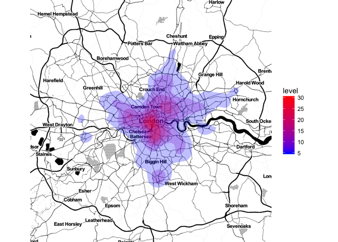
Not bad at all! We can now identify the crime hotspots, but there’s no way we can infer anything about the crime seasonality. And here’s where the first serious use of animated graphs comes in!
CREATING ANIMATED SINGLE-VIEW HEAT MAP
For this purpose I use, now famous, gganimate package. If you ever thought that creating gif’s with changing plots is hard, you’d better start eyeballing the below code, because the only difference between the static and animated graph is frame = Month part added to graph’s aes(). Simples.
#devtools::install_github("dgrtwo/gganimate")
library(gganimate)

map_anime<- ggmap(london_map, extent = "device") +
  stat_density_2d(aes(x = Longitude, y = Latitude, frame = Month,
                      fill = ..level.., alpha=1),
                  data=weapon_map_data, geom = "polygon") +
  scale_fill_gradient(low = "blue", high = "red") +
  scale_alpha(range = c(0.00, 0.5), guide = FALSE)
gganimate(map_anime)
From this animation alone (pretty much) you would know which of the following statements is true: i) weapon-carrying criminals like Easter and summer holidays, thus take time off from their criminal activity during these times and thus reducing the geographical range of such crimes, OR ii) during holiday periods the weapon-carrying criminals tend to ‘focus’ on more central areas, supposedly while keeping up with their criminal activity…?
CREATING ANIMATED MULTIPLE-VIEW HEAT MAP
Following the same logic, we can create a faceted-animated view of all crimes in London over 15 months. It goes like this:
# creating a new data.frame
all_map_data <- london_police_data %>%
  select(Month, Longitude, Latitude, Crime.type)

# animated all london crimes over time
all_london_heat_map<- ggmap(london_map, extent = "device") +
  stat_density_2d(aes(x = Longitude, y = Latitude, frame = Month,
                      fill = ..level.., alpha=1),
                  data=all_map_data, geom = "polygon") +
  scale_fill_gradient(low = "blue", high = "red") +
  scale_alpha(range = c(0.00, 0.5), guide = FALSE) +
  facet_wrap(~ Crime.type, nrow = 3)

gganimate(all_london_heat_map)
So, there you go! At the first glance it may look a bit chaotic, but such visualization will quickly make you realise that some crimes always have a narrow geographical range ( Theft from the person or Other theft, for example), especially compared to some with universally wide range (e.g. Burglary or Criminal damage and arson). And this is the first step for generating new questions and hypotheses, the integral (and very desirable) part of any exploratory analysis!
So, what do you think? Are you converted yet? :)
comments powered by Disqus