Recently, I worked a bit with cluster analysis: the common method in unsupervised learning that uses datasets without labeled responses to draw inferences. I wanted to put my notes together and write it all down before I forget it, thus the blog post. For the start, I’ll tackle multiple approaches to how to determine the number of clusters in your data.
QUICK INTRO
Clustering algorithms aim to establish a structure of your data and assign a cluster/segment to each datapoint based on the input data. Most popular clustering learners (e.g. k-means) expect you to specify the number of segments to be found. However, clusters as such don’t exist in firm reality, so more often than not you don’t know what is the optimal number of clusters for a given dataset.
There are multiple methods you can use in order to determine what is the optimal number of segments for your data and that is what I’m going to review in this post.
I’m not going to go into details of each algorithm’s workings, but will provide references for you to follow up if you want to find out more.
Keep in mind that this list is not complete (for more complete list check out this excellent StackOverflow answer ) and that not all approaches will return the same answer. In such case, my advise would be: try several methods - the more consistency between different approaches, the better - pick the most commonly returned number of clusters, evaluate their consistency and structure (I’ll cover how to do it in the next post) and check if they make sense from the real world point of view.
So there we go!
WINE DATASET
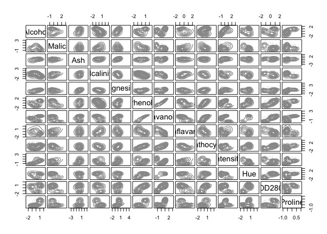
For this exercise, I’ll use a popular wine datasets that you can find built into R under several packages (e.g. gclus, HDclassif or rattle packages). The full description of the dataset you can find here, but essentially if contains results of a chemical analysis of 3 different types of wines grown in the same region in Italy. I’m guessing that the three types of wine (described by Class variable in the dataset) mean white, red and rose, but I couldn’t find anything to confirm it or to disclose which Class in the data corresponds to which wine type… Anyway! Let’s load the data and have a quick look at it:
## loading packages
library(dplyr)
library(knitr)
library(gclus)

# loading data
data(wine)
head(wine) %>% kable()| Class | Alcohol | Malic | Ash | Alcalinity | Magnesium | Phenols | Flavanoids | Nonflavanoid | Proanthocyanins | Intensity | Hue | OD280 | Proline |
|---|---|---|---|---|---|---|---|---|---|---|---|---|---|
| 1 | 14.23 | 1.71 | 2.43 | 15.6 | 127 | 2.80 | 3.06 | 0.28 | 2.29 | 5.64 | 1.04 | 3.92 | 1065 |
| 1 | 13.20 | 1.78 | 2.14 | 11.2 | 100 | 2.65 | 2.76 | 0.26 | 1.28 | 4.38 | 1.05 | 3.40 | 1050 |
| 1 | 13.16 | 2.36 | 2.67 | 18.6 | 101 | 2.80 | 3.24 | 0.30 | 2.81 | 5.68 | 1.03 | 3.17 | 1185 |
| 1 | 14.37 | 1.95 | 2.50 | 16.8 | 113 | 3.85 | 3.49 | 0.24 | 2.18 | 7.80 | 0.86 | 3.45 | 1480 |
| 1 | 13.24 | 2.59 | 2.87 | 21.0 | 118 | 2.80 | 2.69 | 0.39 | 1.82 | 4.32 | 1.04 | 2.93 | 735 |
| 1 | 14.20 | 1.76 | 2.45 | 15.2 | 112 | 3.27 | 3.39 | 0.34 | 1.97 | 6.75 | 1.05 | 2.85 | 1450 |
table(wine$Class)##
## 1 2 3
## 59 71 48Next, I’ll remove the Class variable, as I don’t want it to affect clustering, and scale the data.
scaled_wine <- scale(wine) %>% as.data.frame()

scaled_wine2 <- scaled_wine[-1]

head(scaled_wine2) %>% kable()| Alcohol | Malic | Ash | Alcalinity | Magnesium | Phenols | Flavanoids | Nonflavanoid | Proanthocyanins | Intensity | Hue | OD280 | Proline |
|---|---|---|---|---|---|---|---|---|---|---|---|---|
| 1.5143408 | -0.5606682 | 0.2313998 | -1.1663032 | 1.9085215 | 0.8067217 | 1.0319081 | -0.6577078 | 1.2214385 | 0.2510088 | 0.3610679 | 1.8427215 | 1.0101594 |
| 0.2455968 | -0.4980086 | -0.8256672 | -2.4838405 | 0.0180940 | 0.5670481 | 0.7315653 | -0.8184106 | -0.5431887 | -0.2924962 | 0.4048188 | 1.1103172 | 0.9625263 |
| 0.1963252 | 0.0211715 | 1.1062139 | -0.2679823 | 0.0881098 | 0.8067217 | 1.2121137 | -0.4970050 | 2.1299594 | 0.2682629 | 0.3173170 | 0.7863692 | 1.3912237 |
| 1.6867914 | -0.3458351 | 0.4865539 | -0.8069748 | 0.9282998 | 2.4844372 | 1.4623994 | -0.9791134 | 1.0292513 | 1.1827317 | -0.4264485 | 1.1807407 | 2.3280068 |
| 0.2948684 | 0.2270533 | 1.8352256 | 0.4506745 | 1.2783790 | 0.8067217 | 0.6614853 | 0.2261576 | 0.4002753 | -0.3183774 | 0.3610679 | 0.4483365 | -0.0377675 |
| 1.4773871 | -0.5159113 | 0.3043010 | -1.2860793 | 0.8582840 | 1.5576991 | 1.3622851 | -0.1755994 | 0.6623487 | 0.7298108 | 0.4048188 | 0.3356589 | 2.2327407 |
Keep in mind that many presented algorithms rely on random starts (e.g. k-means), so I set a seed wherever I can so that we have reproducible examples.
Now we can start clustering extravaganza!
DETERMINING THE OPTIMAL NUMBER OF CLUSTERS
1. ELBOW METHOD
In short, the elbow method maps the within-cluster sum of squares onto the number of possible clusters. As a rule of thumb, you pick the number for which you see a significant decrease in the within-cluster dissimilarity, or so called ‘elbow’. You can find more details here or here.
Let’s see what happens when we apply the Elbow Method to our dataset:
set.seed(13)

wss <- (nrow(scaled_wine2)-1)*sum(apply(scaled_wine2,2,var))
for (i in 2:15) wss[i] <- sum(kmeans(scaled_wine2,
                                     centers=i)$withinss)
plot(1:15, wss, type="b", xlab="Number of Clusters",
     ylab="Within groups sum of squares")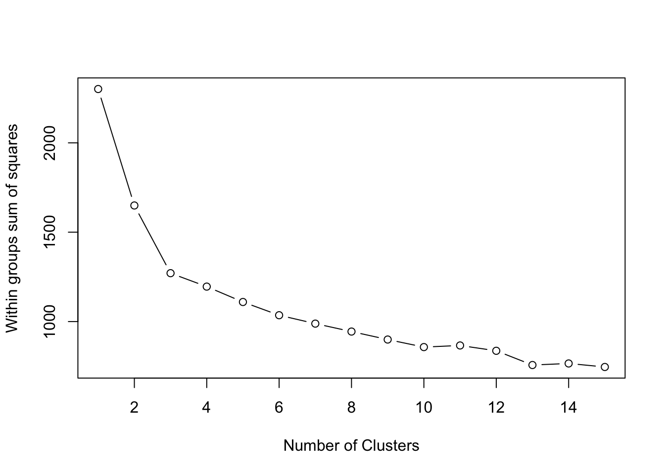
In this example, we see an ‘elbow’ at 3 clusters. By adding more clusters than that we get relatively smaller gains. So… 3 clusters!
2. SILHOUETTE ANALYSIS
The silhouette plots display a measure of how close each point in one cluster is to points in the neighboring clusters. This measure ranges from -1 to 1, where 1 means that points are very close to their own cluster and far from other clusters, whereas -1 indicates that points are close to the neighbouring clusters. You’ll find more details about silhouette analysis here and here.
When we run the silhouette analysis on our wine dataset, we get the following graphs with indication on the optimal number of clusters:
library(fpc)

set.seed(13)

pamk.best2 <- pamk(scaled_wine2)
cat("number of clusters estimated by optimum average silhouette width:", pamk.best2$nc, "\n")
## number of clusters estimated by optimum average silhouette width: 3plot(pam(scaled_wine2, pamk.best2$nc))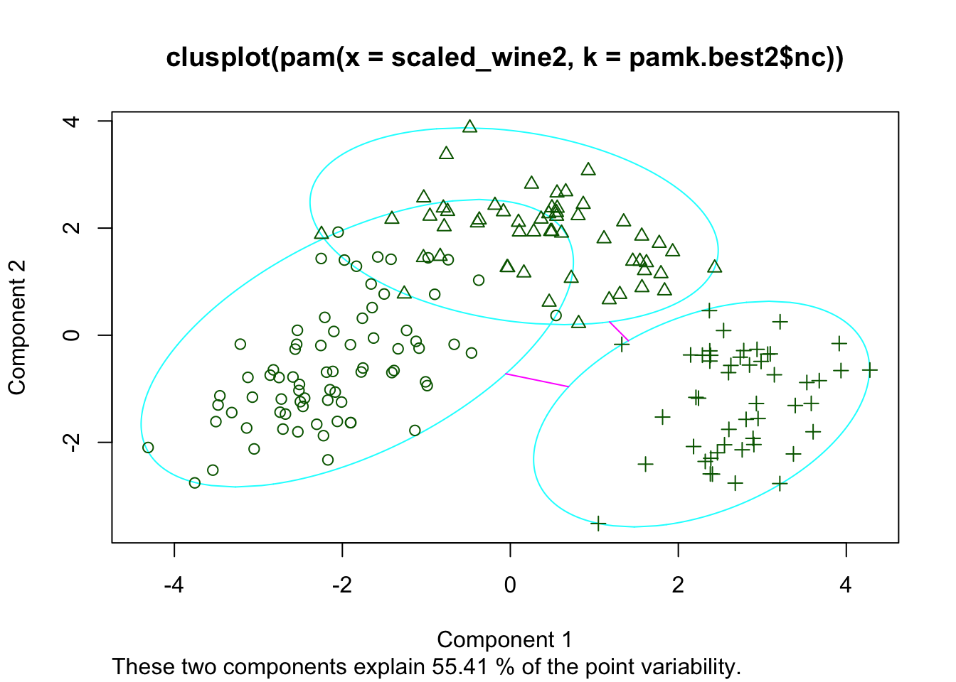
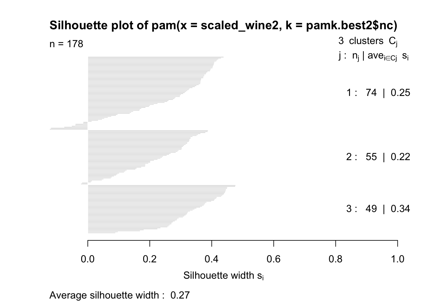
Thus, it’s 3 clusters again.
3. GAP STATISTICS
Gap statistic is a goodness of clustering measure, where for each hypothetical number of clusters k, it compares two functions: log of within-cluster sum of squares (wss) with its expectation under the null reference distribution of the data. In essence, it standardizes wss. It chooses the value where the log(wss) is the farthest below the reference curve, ergo the gap statistic is maximum. Pretty neat!
If you want to know more, check out this presentation for a very good explanation and visualization of what gap statistic is.
Also, for even more details, see the original paper where the gap statistic was first described, it’s like a good novel!
In the case of our wine dataset, gap analysis picks (again!) 3 cluster as an optimum:
library(cluster)

set.seed(13)

clusGap(scaled_wine2, kmeans, 10, B = 100, verbose = interactive())
## Clustering Gap statistic ["clusGap"] from call:
## clusGap(x = scaled_wine2, FUNcluster = kmeans, K.max = 10, B = 100, verbose = interactive())
## B=100 simulated reference sets, k = 1..10; spaceH0="scaledPCA"
## --> Number of clusters (method 'firstSEmax', SE.factor=1): 3
## logW E.logW gap SE.sim
## [1,] 5.377557 5.864072 0.4865153 0.01261541
## [2,] 5.203502 5.757547 0.5540456 0.01356018
## [3,] 5.066921 5.697040 0.6301193 0.01404664
## [4,] 5.033404 5.651970 0.6185658 0.01410140
## [5,] 4.992739 5.616114 0.6233751 0.01342023
## [6,] 4.955442 5.584673 0.6292313 0.01304916
## [7,] 4.933420 5.556602 0.6231820 0.01250233
## [8,] 4.908585 5.531523 0.6229379 0.01299415
## [9,] 4.884336 5.508464 0.6241281 0.01209969
## [10,] 4.858595 5.488182 0.6295870 0.013369104. HIERARCHICAL CLUSTERING
Hierarchical clustering is usually used to better understand the structure and relationships in your data and based on them you decide what number of clusters seems appropriate for your purpose. The way the algorithm works is very well described here and here.
How to choose the optimal number of clusters based on the output of this analysis, the dendogram? As a rule of thumb, look for the clusters with the longest ‘branches’, the shorter they are, the more similar they are to following ‘twigs’ and ‘leaves’. But keep in mind that, as always, the optimal number will also depend on the context, expert knowledge, application, etc.
In our case, the solution is rather blurred:
set.seed(13)

wine_dist2 <- dist(as.matrix(scaled_wine2))   # find distance matrix
plot(hclust(wine_dist2))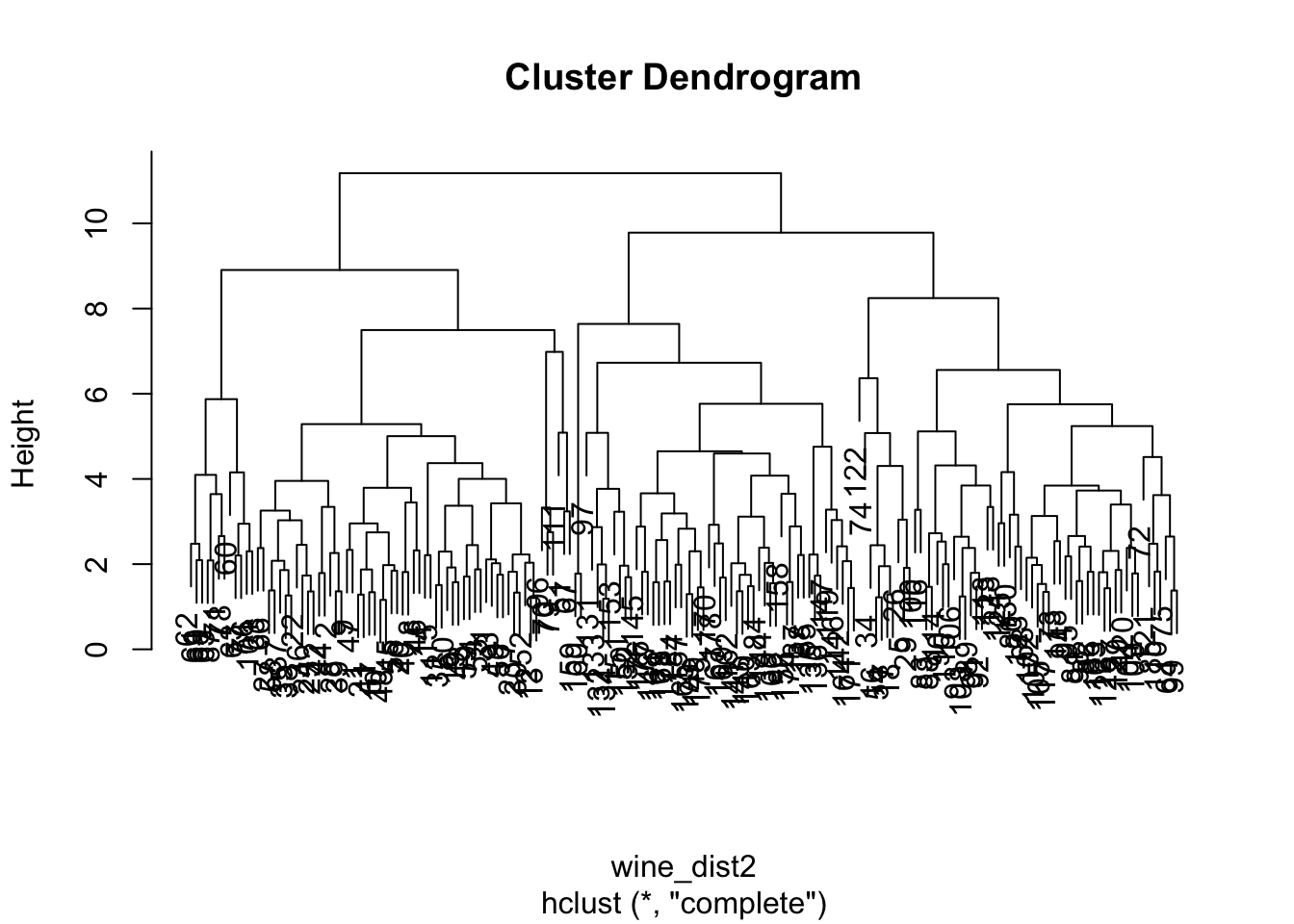
Personally, I would go for something between 2 and 4 clusters. What do you think? :-)
5. CALINSKY CRITERION
yet another method evaluating optimal number of clusters based on within- and between-cluster distances. For more details, see here.
In the example below we set the number of clusters to test between 1 and 10 and we iterated the test 1000 times.
library(vegan)

set.seed(13)

cal_fit2 <- cascadeKM(scaled_wine2, 1, 10, iter = 1000)
plot(cal_fit2, sortg = TRUE, grpmts.plot = TRUE)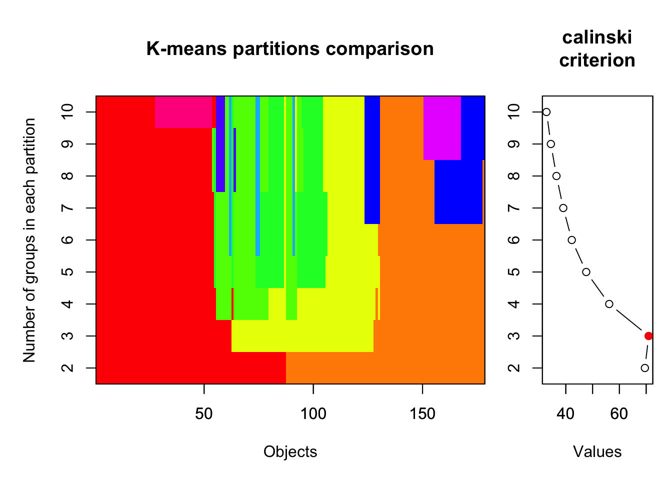
calinski.best2 <- as.numeric(which.max(cal_fit2$results[2,]))
cat("Calinski criterion optimal number of clusters:", calinski.best2, "\n")
## Calinski criterion optimal number of clusters: 3
Again, 3 clusters!
6. BAYESIAN INFORMATION CRITERION FOR EXPECTATION - MAXIMIZATION
This time in order to determine the optimal number of cluters we simultaneously run and compare several probabilistic models and pick the best one based on their BIC (Bayesian Information Criterion) score. For more details, make sure to read this and this.
In the example below, we set the search of optimal number of clusters to be between 1 and 20.
library(mclust)

set.seed(13)

d_clust2 <- Mclust(as.matrix(scaled_wine2), G=1:20)
m.best2 <- dim(d_clust2$z)[2]

cat("model-based optimal number of clusters:", m.best2, "\n")
## model-based optimal number of clusters: 3plot(d_clust2)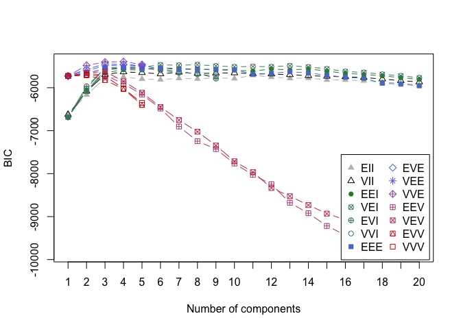
And this time, the optimal number of clusters seems to be 4.
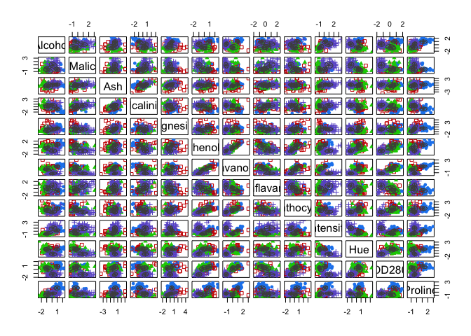
7. AFFINITY PROPAGATION CLUSTERING
I’ll be quite honest with you: I’ve struggled to get my head around what affinity propagation is about! I understood that it clusters data by identifying a subset of representative examples, so called exemplars. And it does so by considering all data points as potential exemplars, but the rest is magic to me..
\[and\] exchanging real-valued messages between data points until a high-quality set of exemplars and corresponding clusters gradually emerges.
(according to Delbert Dueck)
So if you have a better explanation or better materials.. send them over!
In our particular case, this algorithm identified
library(apcluster)

set.seed(13)

d.apclus2 <- apcluster(negDistMat(r=2), scaled_wine2)
cat("affinity propogation optimal number of clusters:", length(d.apclus2@clusters), "\n")
## affinity propogation optimal number of clusters: 15heatmap(d.apclus2)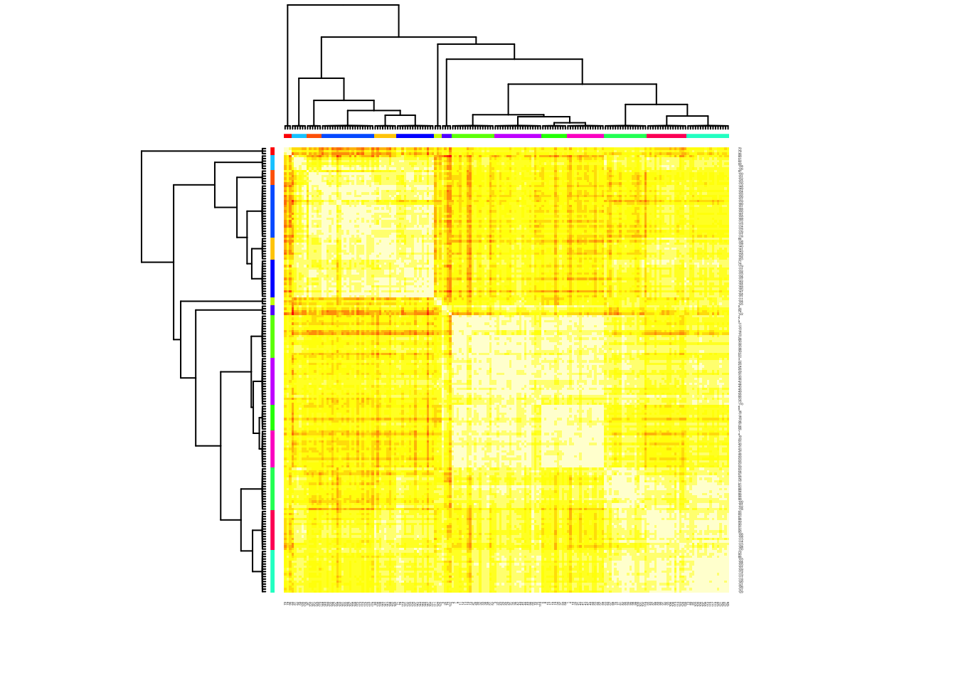
plot(d.apclus2, scaled_wine2)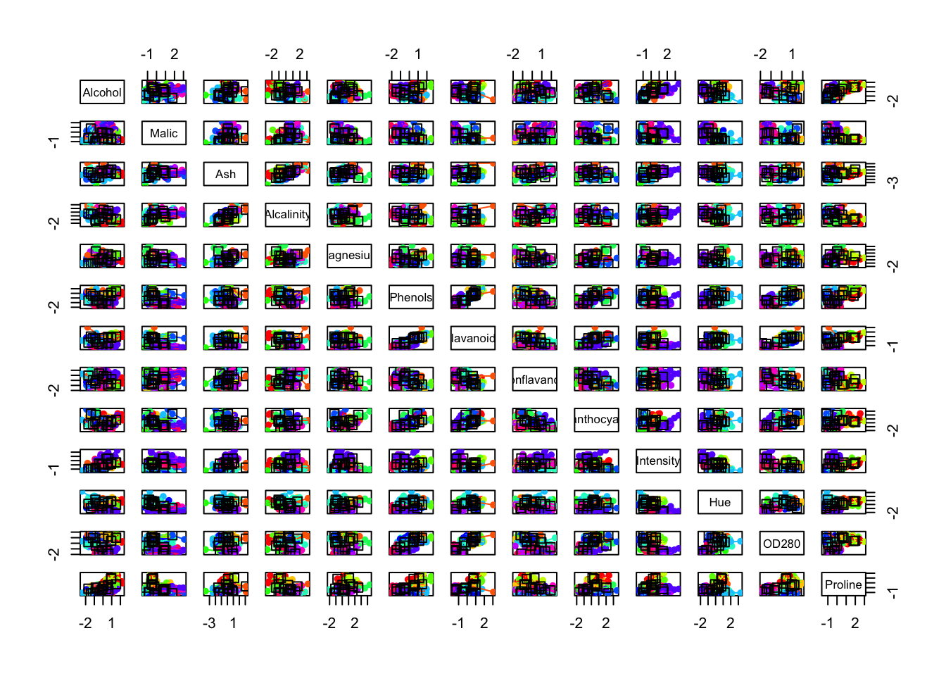
SUMMARY
At least 4 (5, if including hierarchical clustering results) out of 7 tested algorithms suggested 3 as an optimal number of clusters for our data, which is a reasonable way forward, given that the analysed data contained information for 3 classes of wines ;-) In the next post I’ll evaluate those clusters in terms of their stability: how dissolved they are or how often they get recovered.